8 Puzzle
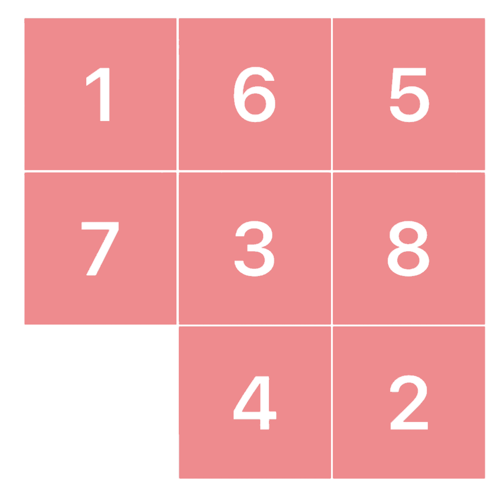
The 8-puzzle game (pictured right) is a classic logical puzzle that consists of a 3x3 grid with eight numbered tiles and one empty space. The objective of the game is to rearrange the scrambled tiles by sliding them into the empty space, ultimately achieving an ordered configuration. As part of my Artificial Intelligence coursework at Case Western Reserve University, I implemented two different agents to solve the 8-puzzle: one using the A* search algorithm and the other utilizing local beam search. In this page, I will discuss the implementation of both agents, the heuristics used for A*, and the results of various experiments conducted to evaluate their performance.
A*:
In my code I represent the puzzle state as an array of arrays which allowed me to easily visualize the puzzle and made it easy to move the blank tile 'b'.
In my implementation of A*, I used two different heuristics. The first, h1, counts the number of tiles that are not in their expected states. This, however, misses many of the nuances of the puzzle, so I also implemented a second heuristic h2. H2, which is also called the Manhattan distance, is the total sum of moves it would take for each tile to return to their goal state, fully unobstructed.
Local Beam:
Beam search, unlike A*, is a local search and is therefore neither optimal, nor complete. This means that beam search is not garunteed to find a solution, and if it does find a solution, it is not garunteed to be the best. However, when beam search does work, it often finds a solution with far fewer nodes generated, albeit usually with a longer path.
Beam search works by picking the k best states, moving in every legal direction for each state, and then by iteratively choosing the k best of the newly generated states. For someone who is familiar with hill climbing, this is essentially the same (pick the best option every time), but with lower odds of reaching a local minima.
Experiments:
After finishing my implementation, I ran a series of experiments to answer a few questions about the performance of the two agents and heuristics.
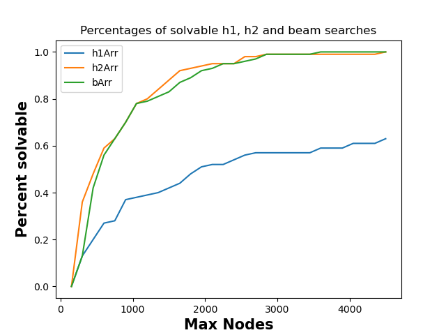
Experiment 1: How does the fraction of solvable puzzles from random initial states vary with the maxNodes limit?
The fraction of solvable puzzles grows as the maxNodes limit grows. This is pretty intuitive, because as you are allowed to generate more nodes for the same puzzle, you could never not solve a puzzle you previously could. To visualize this, I created a function that increments maxNodes from 150 to 4500 with intervals of 150, tested 100 random states and recorded the percentage of solvable puzzles.
Though this graph suggests that beam and h2 generate nodes at a similar level, that is misleading. Beam actually generates far fewer nodes (in general), but encounters more "unsolvable" puzzles, inflating the Max Nodes.
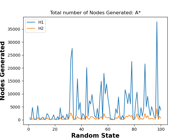
Experiment 2: For A* search, which heuristic is better, i.e., generates a lower number of nodes?
H2 is more efficient than H1 by far. H2 never generates more nodes than H1. This can be viewed by the graph below. It is important to note that H1 and H2 are both optimal and complete heuristics, so they will always find the same solution. This is why they are compared only in efficiency.
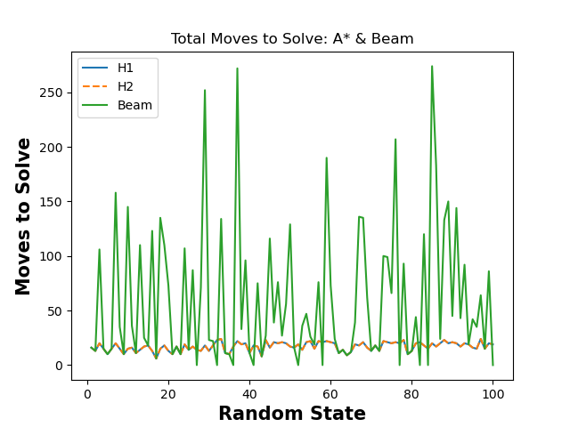
Experiment 3: How does the solution length (number of moves needed to reach the goal state) vary across the three search methods?
The solution for h1 and h2 is always optimal, so the number of moves will never change from one to another. Beam is NOT optimal, so it will always be the same, or worse than A-Star, usually being much worse. This is shown in the below graph. Note: Any time beam is shown lower than h1 or h2 (and only beam is lower), beam search failed to complete with the choice of k, so the total number of moves was set to 0.
Still interested? Check out my GitHub page here!